From MQTT to a live map in Grafana: Helsinki's trams as they move

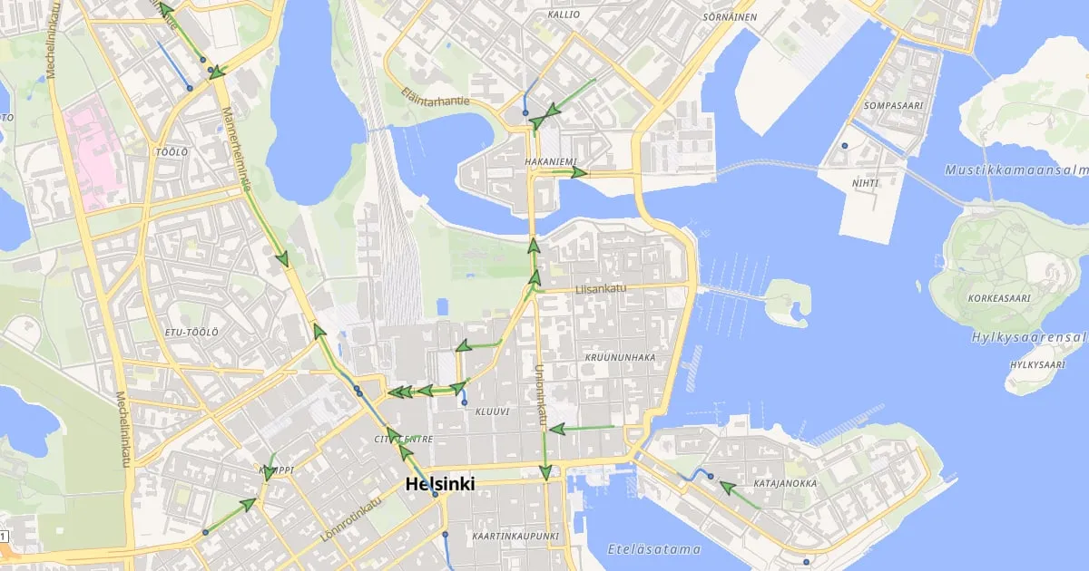
If your vehicles, machines or sensors already publish to an MQTT broker, Grafana can put them on a map. Usually that means a table of positions, or a map that refreshes every few seconds and makes everything jump. This tutorial takes the other road: the map moves each vehicle as its messages arrive, and nothing refreshes.

We use a feed anyone can subscribe to. Every tram, metro, train, ferry and bus of Helsinki Region Transport (HSL) reports its position once a second to a public MQTT broker that needs no key. Follow along on your own Grafana, then point it at your own broker.

What you will build

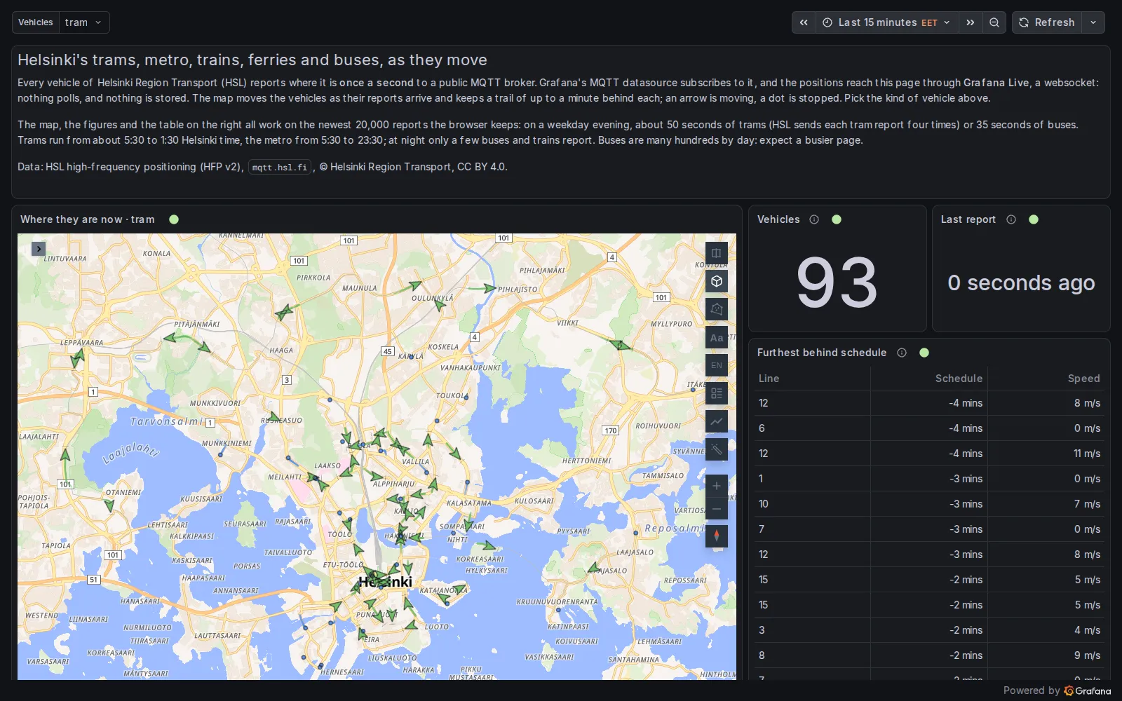
The finished dashboard on 12 November 2026 at 20:15 Helsinki time: 93 trams on the map, the newest report under a second old.

Every tram is on the map, as an arrow pointing where it is going with a short trail behind it, or as a dot when it is stopped. Beside the map, two counters and a table come from the same stream. The live version also switches to the metro, trains, ferries or buses.

You need:

• Grafana 12 (12.0.10 or later).
• Grafana’s MQTT data source, from the catalogue.
• Kepler Geospatial Maps Plus 1.6 or later. That version is the first to move a fleet as a stream arrives.

1. Connect the broker

Add an MQTT data source with this URI, and nothing else:

wss://mqtt.hsl.fi:443/

HSL’s broker needs no user or password. This is MQTT over a websocket on port 443, which gets through firewalls that block MQTT’s own ports. Your own broker may take tcp://, tls:// or ws://, and credentials.

2. Subscribe to a topic

Create a dashboard and add a panel that queries the MQTT data source with this topic:

/hfp/v2/journey/ongoing/vp/tram/#

HSL puts a lot into its topics. Here is one that arrived while we wrote this:

/hfp/v2/journey/ongoing/vp/tram/0040/00075/1002/2/Olympiaterm./19:21/1020446/5/60;24/19/64/82

After vp (vehicle position) come:

• the mode (tram);
• the operator (40) and the vehicle number (75);
• the route (1002, which is line 2) and the direction;
• the destination and the departure time;
• the next stop;
• a geohash of where the tram is.

MQTT’s wildcards can select on any of these levels. # takes everything below it, and + stands for exactly one level. So /hfp/v2/journey/ongoing/vp/tram/+/+/1002/# is line 2 alone, which was five trams when we tried it. A dashboard variable works in a topic too: the live dashboard subscribes to /hfp/v2/journey/ongoing/vp/${mode}/# and switches from trams to buses with a drop-down.

Each message becomes a row with its time and a column VP, which holds the report as JSON. Here is that tram’s report, cut to the keys we use:

{
  "VP": {
    "desi": "2",
    "oper": 40,
    "veh": 75,
    "tst": "2026-11-12T17:40:53.688Z",
    "spd": 0.0,
    "hdg": 85,
    "lat": 60.168863,
    "long": 24.942621,
    "dl": 14
  }
}

• lat and long are the position.
• hdg is the heading, in degrees.
• spd is the speed, in metres per second.
• desi is the line, as passengers know it.
• dl is the offset from the timetable, in seconds. It is negative when the tram is late.

3. Turn messages into rows the map can read

Add three transformations in the panel’s Transform tab:

1. Extract fields: source VP, format JSON, with Replace all fields and Keep time on. Each key of the report becomes a column.
2. Add field from calculation: a binary operation, oper * 100000, alias operator_key.
3. Add field from calculation: operator_key + veh, alias vehicle.

The last two give each vehicle one id, because a vehicle number is only unique within its operator. All the trams belong to operator 40, but the buses don’t: at 19:42 that evening, 43 of the 552 buses on the road shared their number with a bus of another operator. Without the operator, two buses with the same number would be drawn as one bus, jumping across the city. With it, tram 75 of operator 40 becomes 4000075.

Then, in the query options, set Max data points to 20000.

For a streaming query, Max data points is not a resolution. It is how many rows Grafana keeps from the stream, and so how much history the map has for trails. By default it is about the panel’s width in pixels, a thousand rows or so, and HSL’s trams fill that in under three seconds. To size it, multiply your feed’s rows per second by the seconds of trail you want.

When we looked, every tram report arrived four times (bus reports came once each). So 20,000 rows held about 50 seconds of trams.

4. The map

Pick Kepler Geospatial Maps Plus as the visualisation. The data now has an asset (vehicle), a time and a position, so the panel adds a Fleet layer by itself. It also hides the point layer that would draw a dot for every report:

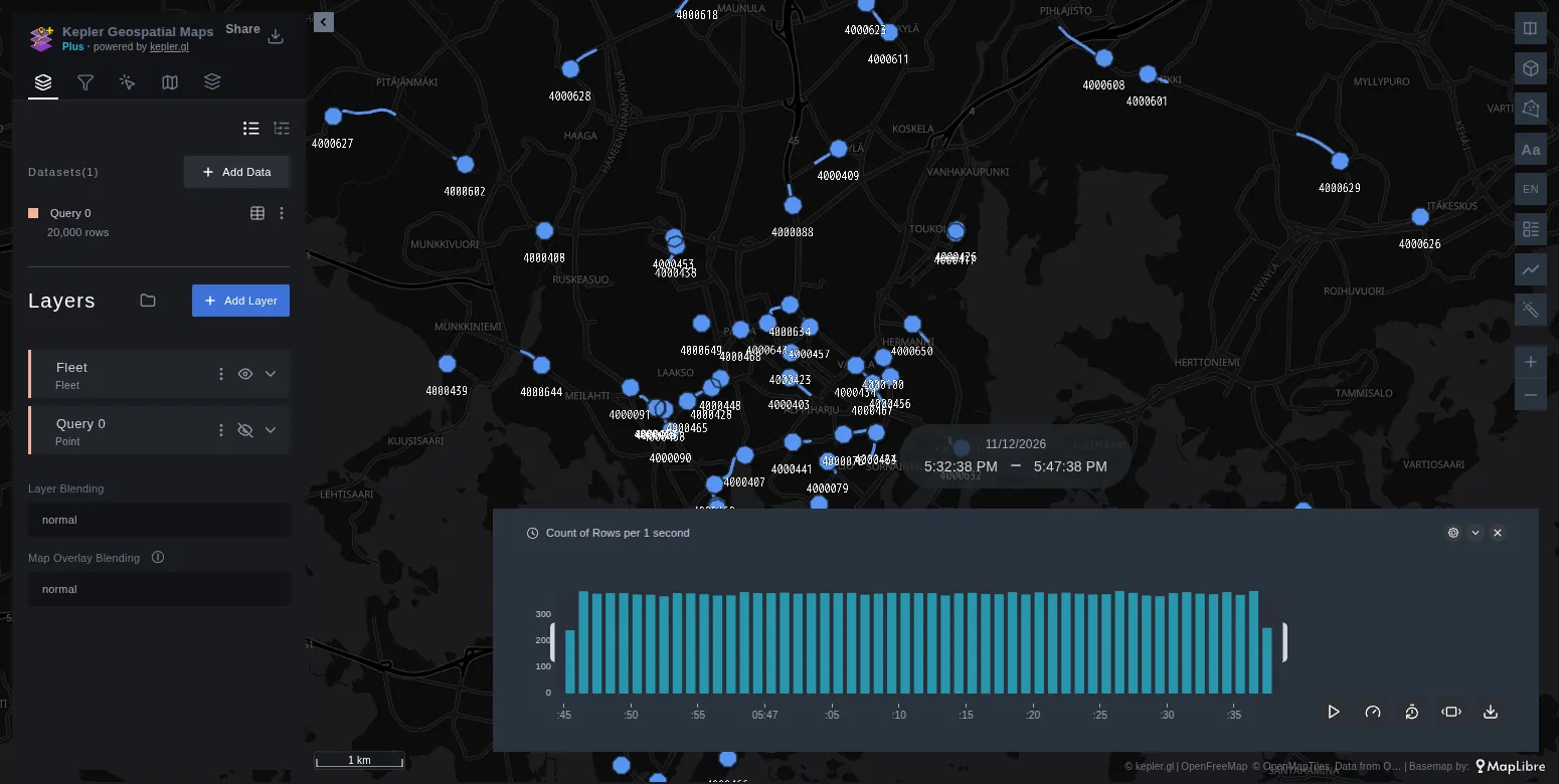
A new panel, with nothing configured yet: a Fleet layer, every tram under its id, and kepler’s time filter along the bottom.

The trams already move. A few settings in the Fleet layer make them easier to read. Each one is named as it appears in the layer panel:

Setting	Value	What it does
Columns → Heading	hdg	turns each tram by its reported heading
Columns → Speed	spd	decides moving or stopped from the reported speed
Stopped below (speed)	2	counts a tram under 2 m/s (about 7 km/h) as stopped
Speed unit	m/s	sets the unit written after the speed on a tram’s card
Marker	Arrow	draws a green arrow when moving and a blue dot when stopped
Label	None	drops the ids, which are noise on a hundred trams; hover one for its card
Trail (min)	1	keeps the trail within the history that Max data points holds
No signal after (min)	2	greys out a tram that has been silent for two minutes

Speed and heading need setting because the panel only recognises them by their usual names: it finds speed or heading by itself, but not spd or hdg. Leave Time reference on Live. Now is then the newest report.

The panel also adds a kepler time filter, with its timeline across the bottom of the map. A live map has little to replay, so you can delete the filter in the Filters tab.

To keep the result, choose Map configuration → Save current map in the panel options, then save the dashboard.

About four minutes of trams in central Helsinki, sped up twenty times. On the dashboard they glide from one report to the next, once a second.

5. Counters and a table from the same stream

The two counters and the table are ordinary Grafana panels. Each one has the same topic and the same first transformations as the map:

• Vehicles: a Group by vehicle transformation, then a Stat panel that counts the rows.
• Last report: a Stat panel on the time column, with the calculation Last and the unit From now. It gives the age of the newest message, the first thing to check when a feed goes quiet.
• Furthest behind schedule: Group by vehicle with the last desi, dl and spd, then Sort by the delay and Limit to 15 rows.

All of this happens in the browser, over what each panel’s buffer holds. Nothing is stored: close the page and it is gone. To keep history, have something write the messages to a database as well, and query that for anything older than the buffer.

When the map stays empty

• Nothing arrives at all. Grafana Live, which carries the stream, is a websocket from the browser to Grafana. Grafana refuses it when the address in the browser is not its root_url and is not listed under [live] allowed_origins. A reverse proxy in front of Grafana also has to pass websocket upgrades. If the browser’s network tab shows /api/live/ws refused, the cause is one of these.
• You get dots instead of a fleet. The panel did not find the asset, the time or the position. Check the column names after the transformations, or set them under Columns in the Fleet layer.
• A saved map lost its layer after you added a transformation. Extract fields renames the dataset that the saved layer points to. Add the Fleet layer again after the transformations, and save the map again.
• Only the last few seconds show. Raise Max data points.

Your own fleet

Nothing here is specific to trams. For a broker of your own, change:

• the URI, the credentials and the topic;
• the transformations, to fit your payload. HSL nests each report under VP, which is why it needs Extract fields. If your ids are already unique, skip the calculation.
• the column names, if you can. A column called vehicle_id, device_id or imei is found as the asset by itself, and heading and speed are found as theirs. The full list is in the Fleet docs.

The Live data guide covers the other way in: Grafana Live push, where anything that can make an HTTP request posts positions to Grafana. Every setting of the dashboard above is in its JSON on GitHub.

Open the live dashboard, pick a mode, and watch Helsinki move.

---

Data. Vehicle positions: HSL high-frequency positioning (HFP v2), © Helsinki Region Transport (CC BY 4.0), documented with every field on Digitransit. Base map: OpenFreeMap, OpenMapTiles, © OpenStreetMap contributors.